PEACH Tutorial
Introduction
"One resembling a peach (as in sweetness, beauty, or excellence)"
Merriam-Webster's Dictionary
"An exceptionally good or attractive person or thing"
Mac OS X dictionary
PEACH (Psychophysics for EACH and every) is a C++ library for programming, running, and analyzing experiments in visual psychophysics. It can also be used for generating visual stimuli for fMRI and EEG/MEG studies. PEACH was designed to be maximally flexible and intuitive to be useful to experienced programmers and novices alike. The library is based on OpenGL, GLUT, and GLUI graphical libraries and runs on Linux and Mac OS X.
Contents
- Hello PEACH!
- Contrast detection experiment
- A retinotopy stimulus
- A search experiment
- Multiple-task and Stereo
- Drawing your own objects
- Improving contrast resolution
- Juicing the data
Hello PEACH!
In this tutorial step you will learn how to:
- put some stimuli on the screen
- compile and run an experiment
- understand the PEACH User Interface (UI) and PEACH output files
- run experiments without the User Interface
Our first experiment is a poor man's experiment. Not much happens on the screen: a greeting appears, and then after a mouse click another message explains how to quit the run. Open you favorite file editor and type/paste there the code shown below, or simply copy the hello_peach.cpp file from the examples directory. The // symbols indicate that any text from there to the line end is comments, not a C++ code. Read the comments!
#include "peach.h"                    // this line links your experiment to the PEACH library

void display()                        // this function defines what is displayed on the screen in each trial
{                                     // it should have no arguments, i.e. the '()'s should be left empty
  Clear();                            // paint the background with the default (black) color
  Text( "Push Esc key to exit", 1. ); // draw the text in white using default size and location
                                      // 'Esc' is the default way to quit an experiment
  Show();                             // display the result on the screen, wait for the observer to respond
}

int main( int argc, char** argv )     // this function prepares and launches the experiment
{                                     // do not rename it; its two arguments are mandatory
  Greeting =                          // defines the text which appears when the experiment starts
    "Hellow PEACH! Push a mouse button to continue";
  SetWindow( argc, argv );            // prepare the main window; the two arguments are mandatory
  Run( display );                     // run the experiment using the function defined above (display)
}
Save the file as hello_peach.cpp. The .cpp extension indicates that this is a C++ file.
Compiling an experiment
Compilation is the process of converting C++ commands into directives for your computer's CPU. To compile the experiment copy Makefile from the PEACH/work directory to the directory where you saved the hello_peach.cpp file (e.g., ~/Work). Open the Terminal window, typecd ~/Work and hit Return. This will put you into the Work directory, which we are going to call "working directory" from now on. Type make, and hit Return. This command will compile all .cpp files in the working directory intelligently: only new files or modified files will be compiled. In our case the make command will create an executable file named hello_peach. Launch the file either by typing its name, e.g., hello_peach in the Terminal window, or by clicking on its icon in the file browser.PEACH user interface
The first to appear is the experiment UI (user interface) window.
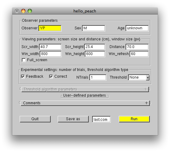
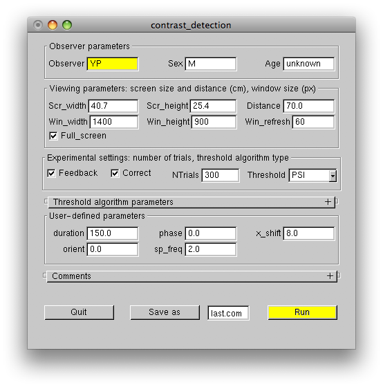
The window contains some default parameters, which you can set or modify before starting the experiment. The Observer parameters panel is self-descriptive. The Viewing parameters panel defines physical dimensions of your screen (Scr_width and Scr_height in cm) and the experimental window dimensions (Win_width and Win_height in pixels). If the Full_screen checkbox is checked, the window will extend to the whole screen. In this case the window parameters will define the screen resolution. Note that the default values of the Scr_width and Scr_height parameters are not accurate, and it is your responsibility to set the correct values for your monitor. The Distance parameter is the viewing distance measured in cm, the Win_refresh parameter defines the screen refresh rate in Hz. This parameter is only effective in the full-screen mode. When using this mode make sure, that the Win_width, Win_height and Win_refresh parameters describe valid monitor settings. When not using the full-screen mode, the screen refresh rate has to be changed using your OS tools. The Experimental settings panel controls auditory feedback (Feedback), finger-error correction (Correct), number of trials (NTrials), and the type of the threshold estimation algorithm to be used (Threshold). The User-defined parameters panel is empty in this experiment, because we did not define any user parameters. The Comments panel used to type in comments can be opened by clicking on the '+' symbol.
To start the experiment click the Run button. This is how the "Hello peach" greeting looks on the screen:
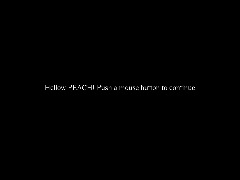
Click any mouse button to proceed. This is the default way to exit the greeting screen. Note that you can also use Left, Down, and Right arrow keys to emulate the left, middle, and right mouse buttons respectively. Push Esc to quit the experiment. If you check your working directory now, you'll find a new file called hello_peach.log. If you take a look at its contents using either a file editor or the more command, you'll find that the file is a complete log of the values that you set using the UI window, as well as other experimental parameters.
PEACH output files
Now launch hello_peach again, and this time change NTrials from 150, which is the default value, to 1. Also, set observer parameters and type some experimental comments. Run the experiment, and this time push either left or right mouse button instead of hittingEsc. This will register a response in the only experimental trial and terminate the experiment in a normal way. Observe that besides the hello_peach.cpp, hello_peach, and hello_peach.log files a new directory named Data has been created. This directory has a file hello_peach_YYMMDD_HHMM.dat, where YYMMDD_HHMM should be your current date and time. If you run the experiment again, another time-stamped .dat file will be created in the Data directory. Unlike the .log file a new .dat file is created for each instance of your experiment. This file contains the experimental settings, as well as the experimental results:
Trial settings: 1 1 1 RANDOM
Video settings: ANG_DEG DST_DEG NO_BLEND VIEW_2D NO_STEREO BITS8 1400x900@60
Experimental settings: SINGLE_TASK TWOAFC
            observer                  YP
                 sex                   M
                 age             unknown
------------------------------------------

Comments: none

Set 0
Config 0
Pc: 0 +/- 0   d':   Bias: -1
The details of the .dat file are explained in the next step of this tutorial.
Bypassing the UI window
Any changes to the UI fields are saved automatically into the .log file, as soon as you hit the Run button. If you wish to prevent observers from making any further changes to the experimental parameters, or you want to run several experiments in a batch, you can disable the UI window and move straight on to the experiment. After setting all the parameters push the Save as button. This will create a command file called last.command in your working directory. You can change its name by typing some other name into the input field next to the Save as button (e.g., my.command). Note that the .command extension is important, because it enables the file to be launched by clicking on its icon in the OS X Finder window. By launching this file you'll start the experiment directly, bypassing the UI window.Back to Contents
Contrast detection experiment
In this tutorial step you will learn how to:
- program a 2AFC experiment
- use the Kontsevitch & Tyler adaptive algorithm and the method of constant stimuli
- estimate psychometric thresholds and their uncertainties
- let observers correct finger errors and initiate trials explicitly
The contrast_detection.cpp example implements a complete contrast detection experiment. The threshold is measured in the 2AFC paradigm using the adaptive algorithm by L. L. Kontsevitch and C. W. Tyler, Bayesian adaptive estimation of psychometric slope and threshold. Vision Res 39, 2729-37 (1999).
#include "peach.h"

void fixation()                                        // this function will be called by the display function
{                                                      // to show the fixation pattern,
  FixationCross();                                     // which consists of the fixation cross
  Circle( -p["x_shift"], 0, 2 / p["sp_freq"], -0.25 ); // and two circles, where the target will appear
  Circle(  p["x_shift"], 0, 2 / p["sp_freq"], -0.25 );
}

void display()
{
  Clear();                                             // clear the screen with the background color
  fixation();                                          // draw the fixation pattern
  Show( 500 );                                         // and display it for 500 msec

  int sgn;
  if( Trial < NTrials / 2 )                            // for the first half of the trials
    {
      sgn = -1;                                        // set the location sign to show the target to the left
      Answer = LEFT;                                   // set the correct answer to the left mouse button
    }
  else                                                 // for the second half of the trials
    {
      sgn =  1;                                        // set the location sign to show the target to the right
      Answer = RIGHT;                                  // and set the correct answer accordingly
    }                                                  // the sequence of trial locations will be shuffled later

  Clear();
  fixation();
                                                       // draw the Gabor target defined by the 'p' array:
  Gabor( sgn * p["x_shift"],                           // specifies the Gabor position along the x-axis
         0,                                            // y = 0 puts the Gabor on the horizontal meridian
         p["orient"],                                  // Gabor orientation wrt the horizontal
         p["sp_freq"],                                 // Gabor spatial frequency in cpd
         p["phase"],                                   // Gabor phase in degrees
         Signal );                                     // 'Signal' contrast is provided by the adaptive algorithm
  Show( p["duration"] );                               // display the target for the user-defined duration in msec

  Clear();                                             // clear the screen
  fixation();                                          // draw the fixation pattern
  Show();                                              // display it and wait for a response
}

int main( int argc, char** argv )
{                                                      // user-defined parameters for this experiment comprise:
  p["orient"] = 0;                                     // the Gabor target orientation
  p["phase"] = 0;                                      // spatial phase
  p["sp_freq"] = 2;                                    // spatial frequency
  p["x_shift"] = 8;                                    // position along the x-axis
  p["duration"] = 150;                                 // stimulus duration in msec

                                                       // the multi-line greeting explains the experimental task
  Greeting = "Fixate at the cross.\n\
A target (Gabor) will appear left/right of the fixation cross.\n\
Respond accordingly with left/right mouse button click.";
  SetTrials( 1, 1, 300, RANDOM );                      // setup an experiment made of 1 set, 1 configuration, 300 trials, and
                                                       // shuffle the 1x1x300 trials randomly
  SetWindow( argc, argv, 0.5, 1, BITS10 );             // setup a window with background color 0.5 (medium gray), gamma 1,
                                                       // 2x2 dithering to produce nominal 10-bit (1024 grays) pixels
                                                       // run the experiment using Kontsevich & Tyler adaptive algorithm (PSI),
  Run( display, PSI, ADAPT_SETS, ADAPT_LOG, 31, .02, 0.1,  31, .02, 0.1,  31, 1., 4. );
                                                       // its parameters specified by ADAPT_SETS, ADAPT_LOG, etc ...
}
The Gabor() function used in this example demonstrates the typical order of a PEACH object parameters. The object position x and y with respect to the center of the screen comes first, the "internal" object parameters, like its orientation and spatial scale come next, and its contrast (color or grayscale) comes last. For each of its RGB components the contrast is defined as the Weber contrast
![\[ \frac{I - I_b}{I_b} \]](form_0.png)
where  is the maximum intensity for a given color component of the object, and
  is the background intensity (defined in the SetWindow() function) for the same component. When applied to Gabor objects
  is taken as the amplitude of the Gabor sine factor, even if this amplitude is not actually present in any of the Gabor pixels due to the Gaussian factor attenuation. When defined in this way the Gabor Weber and Michelson
![\[ \frac{I_{max} - I_{min}}{I_{max} + I_{min}} \]](form_4.png)
contrasts become equivalent:
![\[ \frac{I_{max} - I_{min}}{I_{max} + I_{min}} = \frac{I_b + A - (I_b - A )}{I_b + A + I_b - A} = \frac{A}{I_b} \]](form_5.png)
If the background color component  , than the corresponding contrast parameter is interpreted as the row pixel intensity in the range [0 1]. Negative values are ignored.
Threshold estimation
Compile the code by issuing themake command. After launching the experiment you'll see the experiment's UI window, which now contains the user-defined parameters. Only those parameters which were put into the p array appear in the UI window, all other parameters that you might use in you code remain invisible (e.g., the 500 msec "fixation duration").
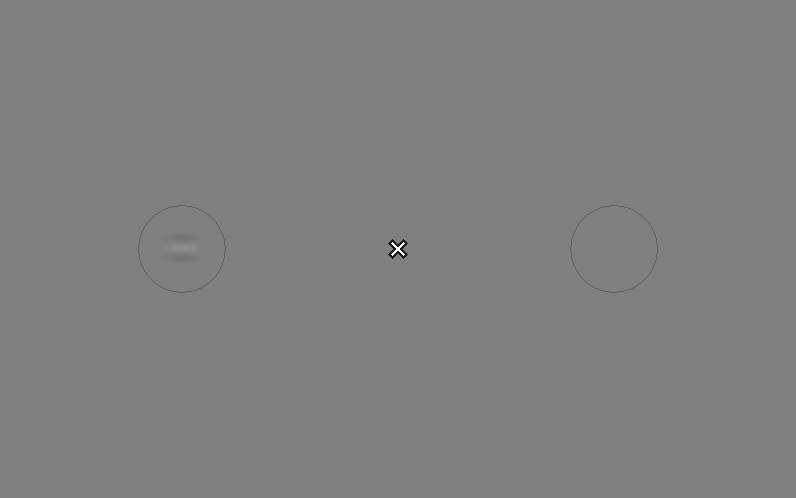
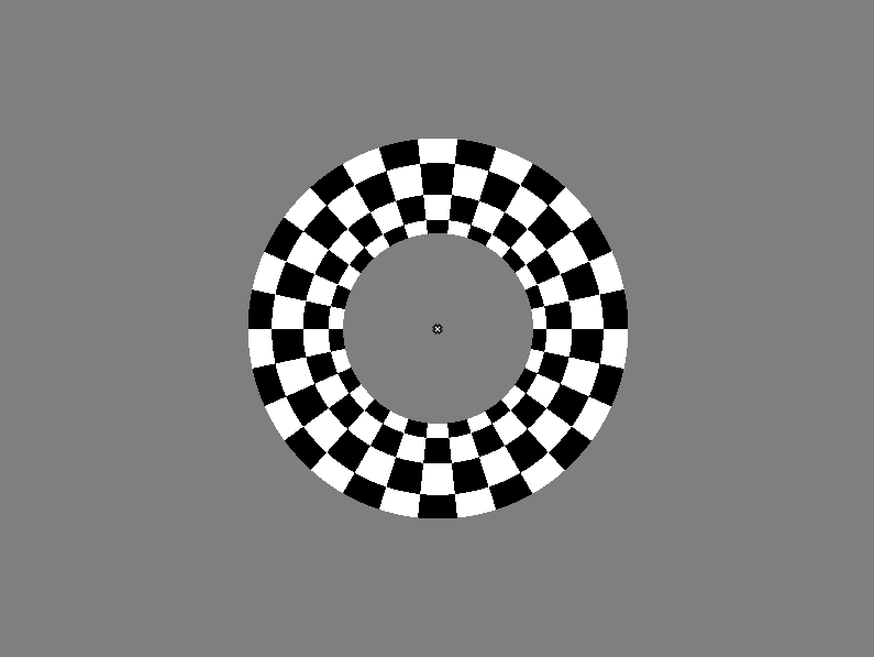
The following figure shows the stimulus with the target Gabor in the left location.
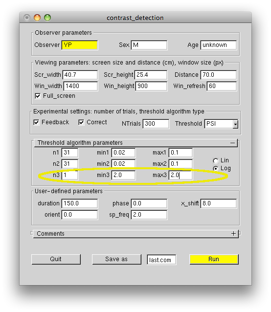
Run the experiment and observe the adaptive fashion in which the target contrast varies. Wrong responses are signaled by the system bell. This auditory feedback can be disabled by unchecking the UI Feedback checkbox. You'll notice that the algorithm tests contrast above and below the threshold contrast most often, which is the optimal way to estimate the slope of the psychometric function. This strategy produces about 75% correct responses on the average. If you wish, you can fix the slope to some value (e.g., 2), by changing the corresponding parameters in the Threshold algorithm parameters panel, as shown:
In this case the algorithm will mostly test contrasts which produce approximately 90% correct responses, which happens to be the "sweet point" for threshold-only estimation. Although the 90% correct regime is more pleasant for an observer and the algorithm will reach a set threshold precision in fewer steps, the measured threshold will be biased, if the slope was fixed at the value significantly different from the actual psychometric slope. Therefore, the fixed-slope regime should only be used after careful measurement of the actual slope for each observer and each experimental task, but is better avoided altogether. As the following figure demonstrates, the precision of the threshold estimate converges very quickly even when the slope is not fixed, and typically 150 trials are enough to get the precision of 10% or better.
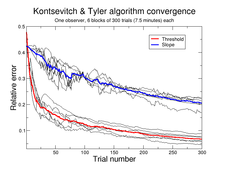
The figure plots the precision of threshold and slope estimates calculated from the adaptive algorithm results. An observer carried out 6 runs of the contrast_detection experiment. The results for individual runs are shown in black. Bold curves show the precision averaged over the six experimental runs. The slope estimate converges slower than the threshold estimate, and approximately 4 times more trials are needed to get the same degree of precision. Thus, 300 trials typically give about 20% precision for the slope estimate.
The Threshold algorithm parameters panel has three rows. The rows hold the same numbers, which followed the PSI, ADAPT_SETS, ADAPT_LOG arguments of the Run() function. The first row contains the target parameters: the number of contrast steps n1, min contrast min1 and max contrast max1 tested by the algorithm. The second and the third rows contain analogous parameters for the 2D distribution of threshold (second row) and slope (third row) estimated by the adaptive algorithm. Normally, the second row has the same parameters as the first row. The number of steps n should be set around 30, unless you want to constraint threshold or slope to just one value.
After running the experiment, you'll find its results printed out into the Terminal window, as well as saved in a time-stamped .dat file inside the Data directory, e.g.:
Trial settings: 1 1 300 RANDOM
Video settings: ANG_DEG DST_DEG NO_BLEND VIEW_2D NO_STEREO BITS10 1400x900@60
Experimental settings: SINGLE_TASK TWOAFC
            observer                  YP
                 sex                   M
                 age             unknown
------------------------------------------
            duration                 150
              orient                  45
               phase                   0
             sp_freq                   2
             x_shift                   8

Comments: none

Set 0
Config 0
Pc: 0.7067 +/- 0.02629   d': 0.7689 +/- 0.1082   Bias: -0.09333
PSI:
0:0:300
thr: 0.03218 +/- 0.002841; slope: 1.953 +/- 0.4402
The line starting with "Pc" gives the proportion of correct responses in the experiment and the response bias. The Pc standard deviation is calculated assuming that the trials are Bernoulli trials. The Bias is calculated as the sum of left (-1) and right (+1) mouse responses divided by the total number of responses. The same line also shows the detectability d' corresponding to the measured Pc. PEACH calculates d' assuming the 2AFC paradigm, as  , where
  is the inverse of the cumulative normal distribution function.
The block starting with "PSI" shows the results produced by the adaptive algorithm: threshold thr +/- its standard deviation (estimated by the adaptive algorithm); slope of the psychometric function +/- its standard deviation. The algorithm produces its own data file with the same time-stamp, but with extension .psi. The file contains a full log of the adaptation procedure:
0   0.0554257 1  0.0411521 0.0198891  2.00559 0.851064
1   0.0554257 1  0.0382177 0.0175633  2.01945 0.855166
2   0.0525306 1  0.0357401 0.0154098  2.03847 0.86099
3   0.0525306 1  0.0337919 0.0135398  2.06141 0.867631
4   0.0497867 1  0.032172 0.0119188  2.08629 0.874133
5   0.0497867 0  0.0482843 0.0184726  1.84086 0.772612

...

297   0.065104 1  0.0421422 0.00271974  2.64806 0.494284
298   0.0341995 1  0.0420108 0.00271506  2.62853 0.492098
299   0.065104 1  0.0419986 0.00271044  2.63291 0.491816

0.0324131     162  108  0.666667 +/-   0.037037
0.0380731      20   15      0.75 +/-  0.0968246
0.0447214       2    1       0.5 +/-   0.353553
0.0525306       4    4         1 +/-          0
0.0617034      88   86  0.977273 +/-  0.0158869
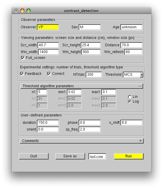
By choosing the MSC option instead of PSI in the Threshold list one switches to the method of constant stimuli, which is not adaptive. Therefore, the algorithm parameters have to be chosen more carefully. The parameters are the number of contrast steps n1, the min min1, and the max max1 of the target contrast:
The output of the MCS algorithm is self-explanatory:
MCS:
0:0:300
Signal     Pcorr +/- stdv    d' +/- stdv       log(d') +/- stdv
 0.040     0.717 +/- 0.058   0.810 +/- 0.245   -0.210 +/- 0.307
 0.045     0.700 +/- 0.059   0.742 +/- 0.242   -0.299 +/- 0.334
 0.051     0.850 +/- 0.046   1.466 +/- 0.286   0.382 +/- 0.193
 0.058     0.833 +/- 0.048   1.368 +/- 0.277   0.313 +/- 0.202
 0.065     0.917 +/- 0.036   1.956 +/- 0.345   0.671 +/- 0.173
Probit:
thr: 0.04554 +/- 0.003331;  slope: 1.844 +/- 0.6254; chi^2: 1.893; P(better fit): 0.405
Note that the MCS algorithm gives a less precise estimate of the psychometric function parameters for the same number of trials, compared to the adaptive PSI algorithm. A benefit of the MCS algorithm is that it samples the psychometric function uniformly and in a controlled fashion, unlike the PSI algorithm.
Correcting finger errors
PEACH provides a simple mechanism to correct accidental mistakes due to "finger errors", i.e., those responses, where a wrong mouse button has been pressed by accident. To correct such a trial the observer has to push the middle mouse button as a response to the next trial. PEACH will ring the system bell three times in a row and then return the experiment to the beginning of the previous trial. This correction option can be disabled by unchecking the UI Correct checkbox.Explicit trial initiation
The default PEACH behavior is to start the next trial, as soon as the observer responds to the previous trial. To let the observer initiate each trial explicitly by pushing the middle mouse button modify the display function as following:
void display()
{
  Clear();
  fixation();
  Show( 500 );

  if( Confirm() == CONFIRM_OK )    // the middle mouse button has to be pressed in order to "confirm" the next trial
    {                              // until then the part of the display function between the curly bracket here...
      int sgn;
      if( Trial < NTrials / 2 )
        {
          sgn = -1;
          Answer = LEFT;
        }
      else
        {
          sgn =  1;
          Answer = RIGHT;
        }
      Gabor( sgn * p["x_shift"], 0, p["orient"], p["sp_freq"], p["phase"], Signal );
      Show( p["duration"] );
    }                              // ... and here will not be executed

  Clear();
  fixation();
  Show();
}
In this case in order to correct a "finger error" the observer has to push the middle button to advance to the next trial and then push it again as a response to this trial. PEACH will return the experiment to the previous trial, where the erroneous response can be corrected.
Back to Contents
A retinotopy stimulus
In this tutorial step you will learn how to:
- present animated stimuli (flicker, drift, etc.)
- store stimuli in video memory for quick rendering
- proceed from trial to trial without waiting for the observer's response
- interleave trials for several experimental conditions within one run
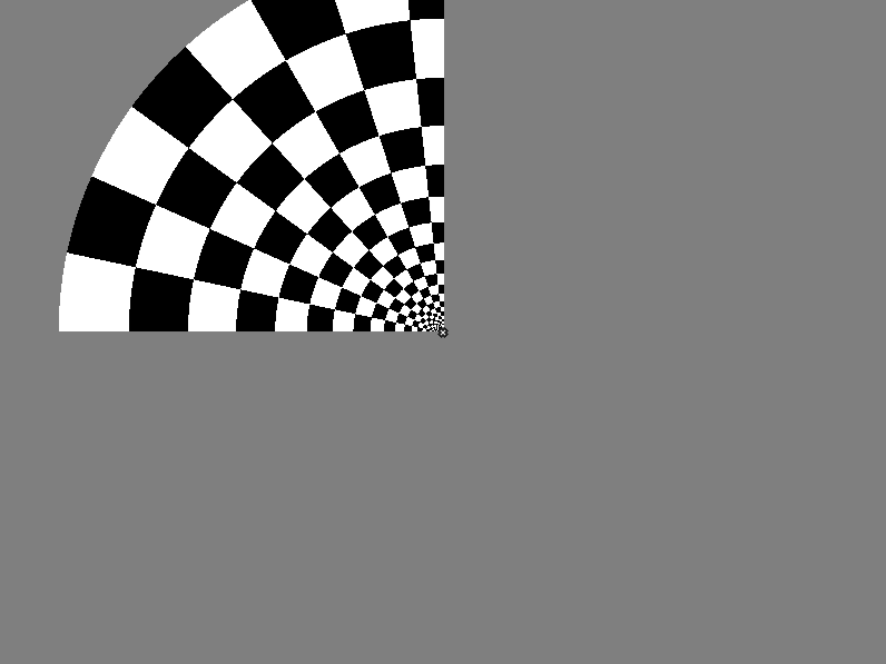
The retionotpy.cpp example implements a typical stimulus for an fMRI retinotopy experiment. First a flickering checkered ring is displayed at four different eccentricities, then a flickering checkered sector is presented at four quadrants of the visual field.
#include "peach.h"

int nSlides, slide_duration;

void display()
{
  Clear();
  FixationCross( 0.2, 1 );                                     // 0.2 deg cross of 100% contrast
  Show( 500 );                                                 // make a 500 msec pause between trials

  for( int i=0; i<nSlides; i++ )                               // loop through the animation slides
    {
      Clear();
      FixationCross( 0.2, 1 );
      Put( Set * 8 + Config );                                 // draw +contrast object
      Show( slide_duration );                                  // show it for one slide duration
      Clear();
      FixationCross( 0.2, 1 );
      Put( Set * 8 + Config + 4 );                             // draw -contrast object
      Show( slide_duration );                                  // show it for one slide duration
    }
}


void prepare()                                                 // this function prepares objects and stores
{                                                              // them as textures in video memory
  nSlides = int( rint( p["duration"] * p["freq"] ) );          // number of slides
  slide_duration = int( rint( 0.5 * 1000 * p["duration"] / nSlides ) );

  int nsectors = int( p["sectors"] );
  MakeCheckeredRing( nsectors, 0, .1, 1.,  1., 0 );                 // prepare rings of four sizes
  MakeCheckeredRing( nsectors, 0, 1., 2.,  1., 1 );
  MakeCheckeredRing( nsectors, 0, 2., 4.,  1., 2 );
  MakeCheckeredRing( nsectors, 0, 4., 8.,  1., 3 );

  MakeCheckeredRing( nsectors, 0, .1, 1., -1., 4 );                 // prepare the same rings of opposite contrast
  MakeCheckeredRing( nsectors, 0, 1., 2., -1., 5 );
  MakeCheckeredRing( nsectors, 0, 2., 4., -1., 6 );
  MakeCheckeredRing( nsectors, 0, 4., 8., -1., 7 );

  MakeCheckeredSector( nsectors, 0, .1, 8., 0.,   90.,   1., 8  );  // prepare sectors for the four quadrants
  MakeCheckeredSector( nsectors, 0, .1, 8., 90.,  180.,  1., 9  );
  MakeCheckeredSector( nsectors, 0, .1, 8., 180., 270.,  1., 10 );
  MakeCheckeredSector( nsectors, 0, .1, 8., 270., 360.,  1., 11 );

  MakeCheckeredSector( nsectors, 0, .1, 8., 0.,   90.,  -1., 12 );  // the same sectors of opposite contrast
  MakeCheckeredSector( nsectors, 0, .1, 8., 90.,  180., -1., 13 );
  MakeCheckeredSector( nsectors, 0, .1, 8., 180., 270., -1., 14 );
  MakeCheckeredSector( nsectors, 0, .1, 8., 270., 360., -1., 15 );
}


int main( int argc, char** argv )
{
  p["duration"] = 1;                                           // stimulus time in seconds
  p["freq"] = 5;                                               // stimulus frequency in Hz
  p["sectors"] = 30;                                           // number of sectors per full circle

  Greeting = "Click any mouse button to start the experiment";

  SetTrials( 2, 4, 5, ORDERED );                               // 2 sets: one for rings, the other for sectors
                                                               // 4 configurations: 4 rings and 4 sectors
                                                               // 5 trials: repeat each trial 5 times
  SetWindow( argc, argv, 0.5, 1 );
  SetObjects( prepare );                                       // prepare all texture objects
  Run( display, NO_RESPONSE );                                 // proceed from trial to trial without
                                                               // waiting for subject to respond
}
Storing objects and drawing from memory
PEACH has two different mechanisms for showing stimuli. The "real-time" mechanism where the stimulus is both prepared and drawn during each experimental trial was illustrated in the previous steps of this tutorial. This mechanism is best suited for objects, which are easy to calculate and are not too extensive, so that they can be drawn fairly quickly. Its advantage is that the stimulus parameters can be changed on the fly, e.g., in an adaptive fashion contingent on the observer's responses in the previous trials. Also, soft-edge objects, e.g., Gauss(), Gabor(), GDisk(), GBar(), etc., are displayed with sub-pixel resolution in this case. There is a different mechanism, which separates the stimulus preparation and the stimulus drawing phases. A pixmap (pixelated image) of an object is prepared before the experimental run starts and is then stored in the computer memory. During the trial the stored pixmap is retrieved from memory and rendered on the screen, which makes it possible to present large and complex stimuli at high temporal frequencies. The downside is that once prepared the pixmap cannot be modified and cannot be positioned on the screen with sub-pixel resolution.Pixmaps are prepared by MakeObject() functions, for example the MakeCheckeredRing() function in the above experiment. MakeObject() function has the same arguments as the corresponding Object() function, except that the first two (x and y) arguments are omitted, and the object's ID argument is added to the end of the argument list. If the object ID is an integer (in the example above it varies from 0 to 15), the object's pixmap is stored in video memory (on the graphics card). In this case the rendering phase is particularly fast. If the object ID is instead a pointer to an array of unsigned short integers (unsigned short*), then the object's pixmap is stored in the computer RAM memory. It takes longer to retrieve a pixmap from the RAM memory, but, on the other hand, the size of RAM memory is usually several times larger than the size of video memory. For example, movies made of thousands of video-frame images can be too large to be stored in video memory, but can be stored in RAM.
The MakeObject() functions used to prepare the stimulus are normally grouped together and put into one function, which in our example was called prepare(). This function is passed as the sole argument to the SetObjects() function, which is executed by PEACH after the Run button is pressed immediately before the greeting message is displayed.
The stored images are drawn on the screen using the Put() function. This function has three arguments: the first two (x and y) define the position of the object inside the experimental window, while the third argument identifies the object. If only the object ID argument is given, the object is positioned in the center of the window.
Multiple experimental conditions in one run
This experiment uses 2 sets, 4 configurations for each set, and 5 trials for each configuration: 2 x 4 x 5 = 40 trials altogether. The ORDERED flag of the SetTrials() function specifies, that the trials will not be shuffled, so that trials, configurations, and sets will follow in order from 0 to 5, 0 to 4, and 0 to 1 respectively. The set number (0 or 1) determines whether a ring or a sector is shown. The configuration number (0 to 4) determines the size of the ring and the quadrant where the sector is drawn. In each trial the positive contrast (+1) checkerboard image alternates with the negative (reversed) contrast image nSlides times, as defined in the display() function. This contrast reversal movie plays five times in a row, as defined by the 5 trials.Experiment without observer responses
The Run() function has the NO_RESPONSE experimental response flag, which starts the next trial as soon as the previous trial ends, without pausing for the observer's response. The default experimental response flag is TWOAFC, which expects Left, Middle, or Right mouse click from the observer after each trial, and will not initiate the next trial until the observer's response is registered. The next tutorial step will demonstrate how to use the other two types of the experimental response flag: POINTER and TIMER.The following figures demonstrate one frame of the experimental stimulus for each set.
for Set = 0, Config = 2:
for Set = 1, Config = 1:
Note that the nSlides and slide_duration variables were set in the prepare() function. It could not be done in the main() function, because the values of the p array could be changed later by user input into the UI window (which is opened after the Run() function executes). These variables could also be calculated in the display() function, which is called in every trial, but because these variables do not change, it was enough to calculate them just once, when the stimulus images were prepared.
Back to Contents
A search experiment
In this tutorial step you will learn how to:
- load and display images
- register response time
- register response location
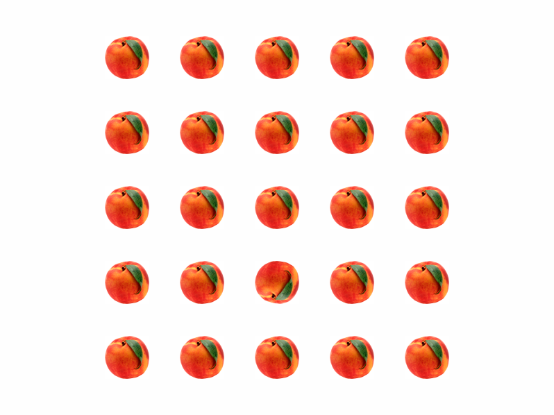
The search.cpp example implements the typical search experiment. A 5x5 array of peach images is presented on each trial, in half of the trials one of the images is shown upside-down. Observer's task is to click the left mouse button as soon as he finds the odd image, or to click the right mouse button if he finds none.
#include "peach.h"

enum{ NORMAL, UPDOWN };                        // alias 0 as NORMAL and 1 as UPDOWN for convenience

double per;

void display()
{
  Clear();
  Show( 1000 );                                // pause to mask the target transition

  Clear();
  for( int i = 0; i < NConfigs; i++ )          // loop over all locations in a 5x5 lattice
    {
      double x = ( i / 5 - 2 ) * per;          // x coordinate (column)
      double y = ( i % 5 - 2 ) * per;          // y coordinate (row )
      if( Set == 0 &&                          // if this is the target set and
          i == Config )                        // Config defines the target location
        Put( x, y, UPDOWN );                   // draw the upside-down image
      else                                     // for all other locations
        Put( x, y, NORMAL );                   // draw the normal side up image
    }
  if( Set == 0 )                               // define what mouse button to use to
    Answer = LEFT;                             // indicate target
  else
    Answer = RIGHT;                            // and no target

  Show();                                      // display until the observer responds
}

void prepare()
{
  per = p["size"] / 4.;                        // calculate the lattice period
  ReadImage( "peach-normal.ppm", NORMAL );     // read the normal side up image
  ReadImage( "peach-updown.ppm", UPDOWN );     // read the upside-down image
}

int main( int argc, char** argv )
{
  p["size"] = 12;                              // stimulus size in degrees

  SetWindow( argc, argv, 1, 1 );               // use white background, gamma = 1
  SetTrials( 2, 25, 10, RANDOM );              // 2 sets (0 - target, 1 - no target), 25 configurations define
                                               // a 5x5 square lattice of images, 10 trials per each location
  SetObjects( prepare );
  Run( display, TIMER );                       // run the experiment and record response times
}
Load and display images
The peach image is loaded by the ReadImage() function. The same as MakeObject() functions ReadImage() can load images into video memory or RAM memory. If the function's last argument is an integer number, the image is loaded into video memory as an OpenGL texture with its ID given by the integer number. If the last argument is a pointer to unsigned char or unsigned short, the image is loaded into RAM memory at the address specified by the pointer. ReadImage() only reads images in ".pgm" (grayscale) or ".ppm" (color) graphical format. This is a simple format convenient for reading and writing uncompressed images. The list of applications that can save images in this format includes Matlab, GIMP, and Linux 'convert' command-line utility. There are also free pgm/ppm plugins for Photoshop.The saved image is drawn on the screen by the same Put() function as for any saved object. In this example a 5x5 lattice of images with one upside-down target image is created, where each of the 25 experimental configurations defines a unique target location within the lattice. For configurations in Set = 1 no target image is shown. The figure shows the stimulus with the target present.
Response time
The TIMER flag for the Run() function indicates that the response time (the time interval between stimulus presentation and the observer response) must be recorded. The output .dat file for this experiment may look like this:
Trial settings: 2 25 10 RANDOM
Video settings: ANG_DEG DST_DEG NO_BLEND VIEW_2D NO_STEREO BITS8 1400x900@60
Experimental settings: SINGLE_TASK TIMER
            observer                  YP
                 sex                   M
                 age             unknown
------------------------------------------
                size                  12

Comments: none

Set 0
Config 0
RT:  828 644 892 564 1348 805 941 933 645 492
Av_RT: 809.2
Pc: 1 +/- 0   d':   Bias: -1
Config 1
RT:  556 557 509 508 620 628 532 581 556 644
Av_RT: 569.1
Pc: 1 +/- 0   d':   Bias: -1
Config 2
...

Config 24
RT:  677 924 685 740 524 820 740 1101 876 1052
Av_RT: 813.9
Pc: 1 +/- 0   d':   Bias: -1

Av_RT: 687
Pc: 0.972 +/- 0.01043   d': 2.703 +/- 0.23877  Bias: -0.944

Set 1
Config 0
RT:  588 484 469 565 621 1068 612 1268 677 701
Av_RT: 705.3
Pc: 1 +/- 0   d':   Bias: 1
Config 1
RT:  437 684 645 788 916 988 885 789 524 1125
Av_RT: 778.1
Pc: 1 +/- 0   d':   Bias: 1
Config 2
...

Config 24
RT:  964 644 525 900 804 596 652 908 693 797
Av_RT: 748.3
Pc: 1 +/- 0   d':   Bias: 1

Av_RT: 822.9
Pc: 0.996 +/- 0.003992   d': 3.751 +/- 1.34741  Bias: 0.992

Av_RT: 755
Pc: 0.984 +/- 0.005611   d': 3.033 +/- 0.20539  Bias: 0.024
The RT: lines show response time for each trial. Also, the average response time (Av_RT), proportion correct (Pc), d', and bias (Bias) for each configuration, set, and for the whole experiment are shown.
Response location
Suppose that we want to modify the search experiment in the following way. The upside-down peach will be presented on all trials now, but after a short exposure (150 msec in this example) all peaches will be replaced by empty squares. The new task is to indicate the upside-down peach location with a mouse click inside the corresponding square. The search-pos.cpp example implements the new version of the experiment:
#include "peach.h"

enum{ NORMAL, UPDOWN };                            // alias 0 as NORMAL and 1 as UPDOWN for convenience

double per;

void display()
{
  Clear();

  for( int i = 0; i < NConfigs; i++ )              // loop over all locations in a 5x5 lattice
    {
      double x = ( i / 5 - 2 ) * per;              // x coordinate (column)
      double y = ( i % 5 - 2 ) * per;              // y coordinate (row )
      if( i == Config ) {                          // Config defines the target location
        Put( x, y, UPDOWN );                       // draw the upside-down image
        AnswerArea[0] = x - 0.45 * per;            // x_min for a correct response
        AnswerArea[1] = x + 0.45 * per;            // x_max for a correct response
        AnswerArea[2] = y - 0.45 * per;            // y_min for a correct response
        AnswerArea[3] = y + 0.45 * per;            // y_max for a correct response
      }
      else                                         // for all other locations
        Put( x, y, NORMAL );                       // draw the normal side up image
    }
  Show( p["duration"] );                           // display for the specified duration

  Clear();                                         // clear the screen and draw a lattice of squares
  for( int i = 0; i < NConfigs; i++ )
    {
      double x = ( i / 5 - 2 ) * per;
      double y = ( i % 5 - 2 ) * per;
      Rectangle( x, y, 0.9 * per, 0.9 * per, -1 ); // draw a square at each location
    }
  Show();
}

void prepare()
{
  per = p["size"] / 4.;                            // calculate the lattice period
  ReadImage( "peach-normal.ppm", NORMAL );         // read the normal side up image
  ReadImage( "peach-updown.ppm", UPDOWN );         // read the upside-down image
}

int main( int argc, char** argv )
{
  p["size"] = 12;                                  // stimulus size in degrees
  p["duration"] = 150;                             // stimulus duration in msec

  SetWindow( argc, argv, 1, 1 );                   // use white background, gamma = 1
  SetTrials( 1, 25, 10, RANDOM );                  // 2 sets (0 - target, 1 - no target), 25 configurations define
                                                   // a 5x5 square lattice of images, 10 trials per each location
  SetObjects( prepare );
  Run( display, POINTER );                         // run the experiment and record response locations
}
The only new elements in this example are the AnswerArea array and the POINTER flag of the Run() function. The latter instructs PEACH to store the screen coordinates of all mouse click responses. The AnswerArea array defines the bounding box for a "correct" mouse click on each trial. The output file contains the coordinates of all the responses, e.g.,
...

Set 0
Config 0
XY:  5.899 6.2 -5.76 -5.483 5.946 3.308 -6.2 -5.899 2.915 -3.262 -2.869 -3.077 -5
.876 -6.362 -6.269 -6.593 -5.552 -5.691 -2.938 -3.447
Av_XY: -2.071,-3.031
Pc: 0.5 +/- 0.1581   d': 0 +/- 0.576   Bias: -1
Config 1
XY:  -5.367 -2.244 -5.853 -2.73 -6.755 -3.493 -6.57 -2.984 -6.316 -3.331 -5.76 -2
.938 -5.83 -2.938 -6.2 -3.123 -6.57 -2.984 -6.478 -2.984
Av_XY: -6.17,-2.975
Pc: 1 +/- 0   d':   Bias: -1
Config 2
...

Config 24
XY:  3.1 2.938 6.293 6.57 5.76 5.622 3.794 6.293 5.76 5.807 -5.205 3.169 6.339 6.
084 3.123 6.478 6.177 3.47 6.616 5.992
Av_XY: 4.176,5.242
Pc: 0.5 +/- 0.1581   d': 0 +/- 0.576   Bias: -1

Av_XY: -0.07764,0.2639
Pc: 0.756 +/- 0.02716   d': 0.9807 +/- 0.1228   Bias: -1
Back to Contents
Multiple-task and Stereo
In this tutorial step you will learn how to:
- display stereoscopic stimuli
- use several tasks for each trial
- combine several experimental and video flags
Stereoscopic presentation
It is easy to display stimuli in stereo, as the hello_peach_stereo.cpp example demonstrates.
#include "peach.h"

void display()
{
  Clear();
  Stereo( SString, 0.,  1., 0.3, string( "Push Esc key to exit" ), 1.,  1,  // Stereo() wraps the SString function
          0.1, 0. );                                // the last two arguments are horizontal and vertical disparities
  Stereo( SString, 0., -1., 0.3, string( "Push Esc key to exit" ), 1., -1,  // the -1 mirror-reflects the text
          -0.1, 0. );
  Show();
}

int main( int argc, char** argv )
{
  Greeting =
    "Hellow PEACH! Push a mouse button to continue";
  SetWindow( argc, argv, 0., 1., STEREO_COLOR_RG );  // STEREO_COLOR_RG flag displays stereo through Red and Green color channels
  Run( display );
}
The SetWindow() function takes the special video flag STEREO_COLOR_RG, which instructs PEACH to display the left eye image in red, and the right eye image in green. The stereogram can be viewed through red-green anaglyphic glasses, or through the Wheatstone stereoscope, after the red and green color channels are split, amplified and displayed onto left eye and right eye monitors. Other stereoscopic options are STEREO_COLOR_RB (red and blue channels), STEREO_SPLIT (the screen is split into left eye and right eye halves), and STEREO_GOGGLES (to be used with shutter glasses, e.g., StereoGraphics CrystalEyes). To display a particular object in stereo, its function has to be wrapped by the Stereo() function wrapper:
Object( arg1, arg2, ... argN );

becomes

Stereo( Object, arg1, arg2, ... argN,   hor_disparity, vert_disparity, eye_flag );
The optional eye_flag can be set to "left" and "right" to display only the left eye and the right eye image respectively. The hor_disparity and the vert_disparity arguments specify horizontal and vertical disparities. The same as for the object's position on the screen, its disparity is measured in degrees of visual angle, unless the DST_PIX video flag is passed to the SetWindow() function, in which case pixel units will be used instead.
The figure shows the hello_peach_stereo stimulus.
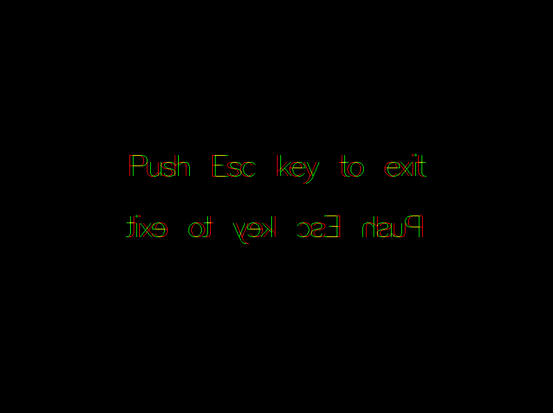
The top and the bottom strings are displayed with opposite disparities. The bottom string is also mirror-reflected, which is handy when viewing the stimulus through a mirror stereoscope. Note that this option is only available for the stencil text function SString(), but not for the bitmapped text used in the Text() function.
Multiple tasks
The contrast_detection_mult.cpp example shows how the contrast_detection.cpp experiment can be modified for two concurrent tasks.
#include "peach.h"

void locators()
{
  Circle( -p["x_shift"], 0, 2 / p["sp_freq"], -0.25 );
  Circle(  p["x_shift"], 0, 2 / p["sp_freq"], -0.25 );
}

void display()
{
  Clear();
  FixationCross( 0.1, 0.2 );
  locators();
  Show( 500 );

  Clear();
  locators();
  Show( 250 );

  int sgn0, sgn1;
  if( Trial < NTrials / 2 )                            // for the first half of trials the target will appear at the left location
    sgn0 =  1;                                         // set the location sign to show the target to the left
  else                                                 // analogously for the second half of the trials
    sgn0 = -1;
  if( ( Trial / ( NTrials / 4 ) ) % 2 == 0 )           // for the first and the third quarter of the trials
    sgn1 = -1;                                         // set the slant sign to the left
  else                                                 // for the other two quarters
    sgn1 =  1;                                         // set the slant to the right

  Clear();
  locators();
                                                       // draw the first Gabor target defined by the 'p' array:
  Gabor( 0,                                            // at the center of the window
         0,
         90 + sgn0 * 20 * SignalMult[ 0 ],             // slanted either left or right off the vertical,
         p["sp_freq"],                                 // the slant controlled by the adaptive algorithm for the first task
         p["phase"],
         0.5 );
                                                       // draw the second Gabor in one of the two locations
  Gabor( sgn1 * p["x_shift"],                          // specifies the Gabor position along the x-axis, etc...
         0,
         p["orient"],
         p["sp_freq"],
         p["phase"],
         SignalMult[ 1 ] );                            // contrast controlled by the adaptive algorithm for the second task
  Show( p["duration"] );

  Clear();
  locators();
  Show( 250 );
}


int main( int argc, char** argv )
{
  p["orient"] = 90;
  p["phase"] = 0;
  p["sp_freq"] = 2;
  p["x_shift"] = 8;
  p["duration"] = 50;

  Greeting = "Fixate at the cross.\n\
Respond to the slant of the central Gabor first\n\
and to the location of the peripheral Gabor second.";
  SetTrials( 1, 1, 300, RANDOM );
  SetWindow( argc, argv, 0.5, 1, BITS10 );
                                                      // note the DUAL_TASK flag threaded together with the PSI flag below
  Run( display, DUAL_TASK | PSI, ADAPT_SETS, ADAPT_LOG, 31, .02, 0.1,  31, .02, 0.1,  31, 1., 4. );
}
The DUAL_TASK flag in the Run() function tells PEACH that the experiment should be set for two concurrent tasks (at most three concurrent tasks are allowed). The first task is to indicate the slant of the central Gabor target (left or right off the vertical), the second task, as before, is to indicate the location of the peripheral Gabor target (left or right). Therefore, two mouse clicks are expected as a response in each trial. The PSI flag in the Run() function ensures that each task is assigned its own instance of the adaptive algorithm. The signals generated by the two instances of the algorithm are retrieved as SignalMult[0] and SignalMult[1]. Note that because both instances of the algorithm are initialized by the same set of threshold algorithm parameters (n1, min1, max1, ...) some scaling may be necessary, if the two adapting parameters are very different. Thus, the SignalMult[0] is scaled by the factor of 20 for the slant of the first target. Accordingly, in order to get the final answer for the slant threshold, the output value of the adaptive algorithm printed into the output file has to be multiplied by the same factor!
Note that no Answer variable was set in the above example, the way it was done in the Contrast detection experiment example. For the dual-task experiment this could be achieved by setting the AnswerMult[0] and AnswerMult[1] to the correct answers (either LEFT or RIGHT). Instead this example demonstrates the default rule for correct answers used by PEACH: LEFT for ODD, RIGHT for EVEN:
- Task 1: the answer is LEFT for first (odd) half of the trials, and RIGHT for the second (even) half of the trials
- Task 2: the answer is LEFT for the first and third quarter of the trials (odd quarters), and RIGHT for the remaining even quarters
- Task 3: the answer is LEFT for the 1st, 3d, 5th, and 7th octals (1/8 groups) of the trials, and RIGHT for the remaining even octals
The output file has the results for the two tasks printed out consecutively for each measurement (Pc, d', Bias, PSI):
Trial settings: 1 1 300 RANDOM
Video settings: ANG_DEG DST_DEG NO_BLEND VIEW_2D NO_STEREO BITS10 1440x900@60
Experimental settings: DUAL_TASK TWOAFC
            observer             YP
                 sex             M
                 age             unknown
------------------------------------------
            duration                  50
              orient                  90
               phase                   0
             sp_freq                   2
             x_shift                   8

Comments: none

Set 0
Config 0
Pc: 0.8267 +/- 0.02185 0.7167 +/- 0.02602   d': 1.331 +/- 0.121 0.8103 +/- 0.1089   Bias: 0 0.04667
Pcc: 0.5833 +/- 0.02846 0.2433 +/- 0.02477 0.1333 +/- 0.01963 0.04 +/- 0.01131
PSI:
0:0:300
thr: 0.03523 +/- 0.003513; slope: 1.084 +/- 0.09527
1:0:300
thr: 0.04074 +/- 0.002702; slope: 2.763 +/- 0.5508
The second threshold (0.04074) multiplied by the factor 20 gives 0.82, which is the slant angle threshold (in degrees) for the first task.
The Pcc: line is a 2x2 matrix, which shows inter-trial correlations between task 1 and task 2 responses averaged over trials. Its first element gives the probability of both responses being true, P(TT), the second element is the probability of the first response being true, and the second response being false, P(TF), the third element is P(FT), and the fourth element is P(FF). This generalizes to a 2x2x2 matrix for the TRIPLE_TASK experiment in the following fashion: P(TTT), P(TTF), P(TFT), P(TFF), P(FTT), P(FTF), P(FFT), P(FFF). As usual, the standard deviations are calculated assuming Bernoulli trial for each response. One can compare the Pcc numbers with simple products of the respective probabilities for each task to see to what degree the responses were correlated between tasks. For example, the simple products of the single-task probabilities (Pc) and their complements (1 - Pc) taken from the above output file would give:
Pcc: 0.5925 0.2342 0.1242 0.0491
By comparing these numbers with the actual Pcc values one can see that they are nearly identical. Therefore, the responses were not significantly correlated between the two tasks.
Flag combinations
As the previous example demonstrates, several Experimental flags for the Run() function, and Video settings flags for the SetWindow() function can be threaded together with the '|' operator, e.g.,
SetWindow( argc, argv, BITS10 | BLEND_TRANSPARENT | STEREO_COLOR_RG );
It is important to understand, that no two settings for a given flag can be combined in this fashion. For example, the TWOAFC (default), TIMER, POINTER, and NO_RESPONSE settings for the experimental response flag are mutually exclusive, and
is not allowed. The NO_STEREO (default), STEREO_SPLIT, STEREO_COLOR_RG, STEREO_COLOR_RB, STEREO_GOGGLES alternative stereo flag settings provide another example.Back to Contents
Drawing your own objects
MakePattern() function
Although PEACH comes with a variety of pre-defined graphical objects in its Objects module (Disks, Bars, Gabors, and like), sooner or later you'll need an object, which is not in the library. One way to deal with this problem is to use the MakePattern() function. This function allows you to create a pixmap stored in RAM or a texture stored in video memory, defined by an arbitrary function f(x, y). PEACH interprets the function output as a contrast profile (color or grayscale), and therefore the function should return a floating number within [-1 1] range. If you wish, you can also return values outside of this range to create transparent areas. The doughnut.cpp example demonstrates the use of the MakePattern() function:
#include "peach.h"

double doughnut( double x, double y )    // this function describes a parabolical surface
{
  double cs = cos( Pi * p["angle"] / 180. );
  double sn = sin( Pi * p["angle"] / 180. );
  double xt =              (  x * cs + y * sn ) / ( 0.5 * p["size"] );
  double yt = p["ratio"] * ( -x * sn + y * cs ) / ( 0.5 * p["size"] );

  return 2 * ( xt * xt + yt * yt - 1 );  // only values within the [-1 1] range will be displayed
}

void display()
{
  Clear();
  Put( 1 );
  Show();
}

void prepare()
{                                        // make a doughnut with maximum red-green contrast
  MakePattern( p["size"], p["size"], doughnut, -p["contrast"], p["contrast"], 0, 1 );
}

int main( int argc, char** argv )
{
  p["size"] = 6.;                        // size of the pattern in degrees
  p["ratio"] = 2;                        // x/y elongation ratio
  p["angle"] = 45.;                      // slant angle in degrees
  p["contrast"] = 1.;                    // the pattern's contrast

  Greeting = "Push a mouse button to view the doughnut";
  SetWindow( argc, argv, 0.5, 0.5, 0. ); // use yellow background
  SetObjects( prepare );
  Run( display );
}
The resulting doughnut shaped object is shown below.
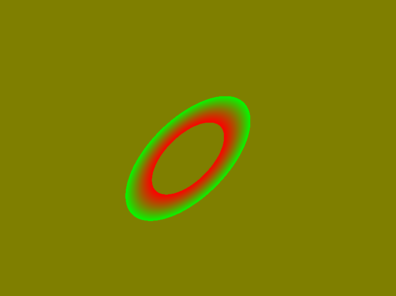
Note that although the doughnut() function defines a complete parabolic surface, only the part of the surface within [-1 1] range is displayed. The rest of the surface (inside and outside of the doughnut) is transparent.
OpenGL capabilities
Because PEACH library is a superset of OpenGL, GLU, and GLUT graphical libraries, you can easily exploit these libraries to create complex 3D objects and scenes. Consult OpenGL User Guide and GLUT User Guide for further references. The teapot.cpp is a simple example of incorporating a 3D object into your experiment:
#include "peach.h"

void display()
{
  Clear();
  glutSolidTeapot( p["size"] * Cm2px );                   // draw the GLUT teapot, its size given in pixels
  Show();
}

void prepare()
{
  GLfloat light0_ambient[] =  { 0.1f, 0.1f, 0.3f, 1.0f }; // setup light characteristics
  GLfloat light0_diffuse[] =  { .6f, .6f, 0.6f, 1.0f };
  GLfloat light0_position[] = { 10.0 * Cm2px, 10.0 * Cm2px, 10.0 * Cm2px, 0.0 };  // setup light position

  glEnable( GL_LIGHT0 );                                  // add the light source
  glLightfv( GL_LIGHT0, GL_AMBIENT, light0_ambient );
  glLightfv( GL_LIGHT0, GL_DIFFUSE, light0_diffuse );
  glLightfv( GL_LIGHT0, GL_POSITION, light0_position );
}

int main( int argc, char** argv )
{
  p["size"] = 6.;                                         // size of the teapot in cm
  Greeting = "Push a mouse button to view the TEAPOT!\nIf you DO NOT wish to see the teapot push Esc.";
  SetWindow( argc, argv, 0., 1., VIEW_3D_PERSP );         // use perspective projection
  SetObjects( prepare );
  Run( display );
}
A light source is created to illuminate the teapot. The VIEW_3D_PERSP video flag specifies that the perspective projection will be used to project the 3D object onto the screen plane. The observer (camera) is set at the ViewingDistance in front of the screen. Thus, the teapot appears in the center of the screen sized according to its physical "size" parameter and the ViewingDistance parameter. Note that only depth values between -0.9 * ViewingDistance and 100 * ViewingDistance are valid when the VIEW_3D_PERSP flag is used. These values correspond to drawing starting from 1/10 of the way between the observer and the screen to 100 times the viewing distance beyond the screen plane. You can use the Cm2px flag to convert physical units to pixel units used by OpenGL. Alternative settings for this flag are VIEW_3D_ORTHO (orthographic projection) and VIEW_2D (2D image), which is the default flag setting.
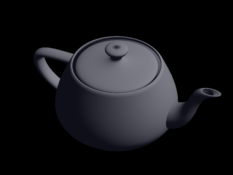
To view the teapot from the angle shown in the figure hold Shift key and drag your left mouse button over the screen to rotate the image into the appropriate position. You can also translate it along the screen plane by using your right mouse button in the same fashion, or zoom on and off the image by using the middle mouse button. If you want more controlled manipulations first push either of the '1', '2', '3', 'x', 'y', 'z' keys (1, 2, 3 stand for roll, pitch, heading) and then adjust the modified parameter by repeatedly pushing either '-' or '+' key.
3D functionality of OpenGL can be useful for creating 2D stimuli. The rotation_expansion.cpp example shows how the stimulus (a random dot pattern here) rotation or expansion can be easily implemented using OpenGL camera motion.
#include "peach.h"

int nSlides, ndots;
double** dots;

void drawDots()
{
  Clear();
  glBegin( GL_POINTS );                     // start drawing the dots
  for( int i = 0; i < ndots; i++ )
    glVertex3f( dots[i][0], dots[i][1], dots[i][2] ); // draw a dot
  glEnd();                                  // stop drawing the dots
}

void display()
{
  double d = 0;
  for( int s = 0; s < nSlides; s++ ) {      // loop through the animation slides
    if( p["condition"] == 0 ) {             // rotation, implemented by rotating the camera
      glPushMatrix();                       // save the current camera position
      glRotatef( d * p["speed"] * 0.1, 0, 0, 1 ); // rotate the camera about the z-axis
      drawDots();
      glPopMatrix();                        // return to the saved camera position
    }
    else {                                  // expansion, implemented by moving the camera
      glPushMatrix();                       // remember the current camera position
      glTranslatef( 0, 0, d * p["speed"] ); // move the camera along the z-axis
      drawDots();
      glPopMatrix();                        // return to the saved camera position
    }

    if( s < nSlides/2 )                    // switch the direction of motion half-way
      d++;
    else
      d--;

    SwapBuffers();                         // display the current slide
  }
}


void prepare()
{
  nSlides = int( rint( p["duration"] * WinFramerate() / 1000. ) );  // number of slides

  ndots =  int( p["n_dots"] );
  dots = new double*[ ndots ];              // allocate ndots x 3 coordinates array
  for( int i = 0; i < ndots; i++ )
    dots[i] = new double[ 3 ];

  for( int i=0; i<ndots; i++ ) {            // generate random dot coordinates
    dots[i][0] = Fran( p["field_size" ] * Deg2px ) - 0.5 * p["field_size" ] * Deg2px; // x
    dots[i][1] = Fran( p["field_size" ] * Deg2px ) - 0.5 * p["field_size" ] * Deg2px; // y
    dots[i][2] = 0;                         // depth coordinate set to the screen surface
  }

  glEnable( GL_POINT_SMOOTH );              // enable OpenGL dot antialiasing
  glHint( GL_POINT_SMOOTH_HINT, GL_NICEST );// of the best possible kind
  glPointSize( 5 );                         // set the OpenGL point size

  MaskCircle( 0, 0, 0.5 * p["field_size" ], OUTSIDE );  // create a circular aperture in the center of the screen

  glEnable( GL_LIGHT0 );                    // add the light source
  GLfloat light_position[] = { 0, 0, ViewingDistance * Cm2px, 0.0 };  // setup light position at observer's position
  glLightfv( GL_LIGHT0, GL_POSITION, light_position );

  double l = p["luminance"];
  GLfloat mat_diffuse[] =  { l, l, l, 1 };  // setup OpenGL material color when lighted from all around
  glMaterialfv( GL_FRONT_AND_BACK, GL_DIFFUSE, mat_diffuse );
}


int main( int argc, char** argv )
{
  p["condition"]   = 0;                     // rotation (0) or expansion (1)
  p["duration"]    = 2000;                  // stimulus time in msec
  p["n_dots"]      = 1000;                  // number of random dots
  p["field_size" ] = 20;                    // field size in deg
  p["speed" ]      = 20;                    // motion speed
  p["luminance"]   = 0.5;                   // dot luminance

  Greeting = "Click a mouse button or press any key";

  SetTrials( 1, 1, 100, ORDERED );
  SetWindow( argc, argv, 0., 1, VIEW_3D_PERSP );         // use perspective viewing
  SetObjects( prepare );                                 // prepare the dot field
  Run( display, NO_RESPONSE | NO_FEEDBACK | NO_CORRECT ); // proceed from trial to trial without
                                                         // waiting for subject to respond
}
Besides the new OpenGL commands the code demonstrates several new techniques. The animation of the random dot motion is created by drawing a frame and swapping the "back" buffer (where the drawing is prepared) with the "front" buffer (rendered on the screen) using the SwapBuffers() function. This renders the drawing on the screen in the very next videoframe. The SwapBuffers() function should be used instead of Show() function when the stimulus duration is on the scale of one video-frame or when a precision of one video-frame is required. To show a stimulus for n video-frames use the SwapBuffers() function inside a loop of n iterations. The WinFramerate() function can be used to calculate the number of video-frames given the stimulus duration in msec. The MaskCircle() function creates a circular aperture which occludes any stimulus beyond the aperture radius. This function can also be used to create a circular occlusion instead. Occluders of other shapes can be created using related masking functions.
Back to Contents
Improving contrast resolution
The following experiments demonstrates the use of the contrast resolution flags BITS8 (default), BITS10, and BITSPP and also give an example of how the user parameters can be validated.
#include "peach.h"

double ramp( double x, double y )  // this function describes a luminance ramp
{
  if( p["size"] <= 0 )
    Error( "You entered the size parameter " +
           F2S( p["size"] ) +
           ".\nThe size parameter should be > 0!" );
  else
    if( fabs( x ) < p["size"] / 2. &&
        fabs( y ) < p["size"] / 2. )
      return x / ( p["size"] / 2. );
  return -2;   // this value (not displayed) is returned to prevent a compiler warning
}

void display()
{
  Clear();
  Put( 1 );
  Show();
}

void prepare()
{                                        // make a doughnut with maximum black-white contrast
  MakePattern( p["size"], p["size"], ramp, p["contrast"], 1 );
}

int main( int argc, char** argv )
{
  p["size"] = 8.;                        // size of the pattern in degrees
  p["contrast"] = 0.2;                    // the pattern's contrast

  Greeting = "Push a mouse button to view the ramp";
  SetWindow( argc, argv, 0.15 ); // use no dithering
  //SetWindow( argc, argv, 0.15, 1, BITS10 ); // use 2x2 dithering
  //SetWindow( argc, argv, 0.15, 1, BITSPP ); // use BITSPP dithering
  SetObjects( prepare );
  Run( display );
}
In the above ramp.cpp code the MakePattern() function calls the user function ramp(), which first validates the 'size' parameter (it should be larger than zero) and defines a horizontal luminance ramp. The Error() function informs the user when the provided size parameter is improper. To see the validation in action run the ramp experiment and set the size parameter to zero. The execution is aborted and the following message appears in the terminal window:
...
ERROR in ramp: You entered the size parameter 0.
The size parameter should be > 0!
Exit 1
Note the use of the F2S() function, which converts a floating-point number to a string of characters.
The ramp.cpp experiment demonstrates how the default 8-bit per color resolution of standard video-cards can be improved using the dithering technique. There are three lines calling the SetWidnow() function in ramp.cpp. The only uncommented line calls the SetWindow() function without any video flags, which means that, by default, the BITS8 video flag is used. Run the ramp experiment with the 'contrast' parameter set to 0.2. The resulting luminance ramp is shown in the left image below.
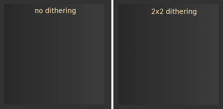
One can notice the faint vertical stripes (Mach bands) arising due to the simultaneous contrast at artefactual luminance boundaries. The luminance boundaries happen wherever the luminance of the ramp reaches one of the luminance levels actually provided by the 8-bit pixel depth of standard video cards. The maximum number of the supported luminance levels is  for each of the 3 color channels and thus the grayscale ramp is actually displayed as a staircase made of distinct luminance grades. The number of grades is even less than 128 if the gamma correction is used, because in this case several lumianance 'steps' might collapse into one.
This pixel-depth limitation is particularly crucial for contrast detection/discrimination experiments, where the contrast increments and decrements are small. To overcome this limitation PEACH provides the BITS10 video regime, which increases the effective pixel depth to 10 bits (1024 luminance gradations). In this regime 2x2 blocks of neighboring pixels are used to create "super-pixels", which increases the number of available luminance levels 4-fold. Accordingly, the effective spatial resolution of the screen is reduced 2-fold in each dimension. Given large enough screen resolution and viewing distance (e.g. 1600x1200 pixels on 21' monitor viewed from 40 cm or more) any artifacts of the 2x2 dithering are well beyond the resolution of the human visual system and are not visible.
To see the dithering in action comment out the first SetWindow() line and uncomment the second line with the BITS10 flag. Compile the changed code (issue the 'make' command) and run the experiment again. The resulting ramp is shown in the right image in the above figure. Thanks to the extra luminance gradations created by dithering the Mach bands are not visible and the ramp appears perfectly smooth.
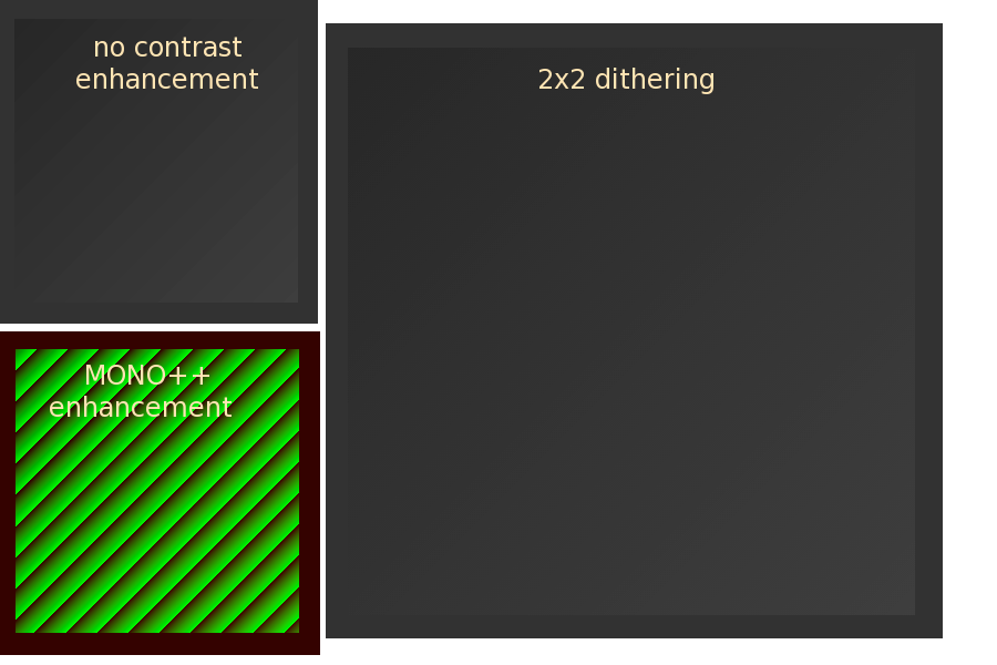
The last commented out line calls the SetWindow() function with the BITSPP flag. This flag implements the MONO++ regime of the BITS++ device manufactured by Cambridge Research Systems. This little but costly piece of hardware is plugged in between the video-card and the monitor and provides 14 bits gray-scale pixel depth without any loss of spatial resolution (at the expense of loosing one color channel). Note that without the device the window created with the BITSPP flag will appear red and green.
The contrast resolution flags can also be used when reading images with the ReadImage() function. The ramp_image.cpp experiment reads the image of a diagonal luminance ramp and displays it on the screen.
#include "peach.h"

void display()
{
  Clear();
  Put( 1 );
  Show();
}

void prepare()
{
  ReadImage( "ramp8.pgm", 1 ); // read a grayscale 8 bit-depth image
  //ReadImage( "ramp16.pgm", 1 ); // read a grayscale 16 bit-depth image
}

int main( int argc, char** argv )
{
  Greeting = "Push a mouse button to view the ramp";
  SetWindow( argc, argv, 0.15 ); // use no dithering
  //SetWindow( argc, argv, 0.15, 1, BITS10 ); // use 2x2 dithering
  //SetWindow( argc, argv, 0.15, 1, BITSPP ); // use BITSPP dithering
  SetObjects( prepare );
  Run( display );
}
Note that BITS10 flag does not eliminate the Mach bands in the "ramp8.pgm" image, because the image has only 8 bits pixel-depth and therefore there is no higher-bit information that dithering could render to improve the image smoothness. By uncommenting the ReadImage() line which reads the "bits16.pgm" image the ramp is redered smoothly with BITS10 flag because this image file stores 16 bits per pixel. The following figure shows the ramp image for the three flag settings: BITS8 (no enhancement), BITS10 (2x2 dithering), and BITSPP (MONO++ enhancement). The latter image is shown how it appears on the screen without the BITS++ device attached.
When images are loaded with the BITS10 regime enabled their size is increased two-fold in each dimension due to the 2x2 pixel dithering. Note that this is not the case for objects and patterns generated by PEACH, their size is kept constant for all contrast resolution flags.
Juicing the data
As you saw, PEACH stores the complete experimental session information in a simple human-readable format inside .dat files. The files are stored in the Data folder, which is created automatically. After running several experimental blocks of several conditions each on several observers the amount of experimental data in the database will build up quickly. The juice command-line utility was designed to reduce the tedious task of manually opening multiple data files and analyzing their contents for different types of measurements. Essentially, it "slices" through the database in a controlled fashion and averages data where possible. The utility is written in Perl, which is a computer language optimally designed for various text processing tasks. Because Perl is the interpreted language, no compilation is required to use it. Just typejuice in the command line of your terminal, and if the PATH variable was set correctly during the PEACH installation, you'll see the juice usage instructions printed out to the screen:
Usage: juice subject_id target_var (i.e. Pc/Bias/thr/slope) file_list (can include wild cards, e.g. *)
For example, juice YP thr asym_mask_070601_*.dat
Several subjects can be included in subject_id using slashes, e.g., YP/OM/PV.
To exclude certain files from the *-wildcarded list append the names of the files with a minus sign
attached to the name of each file, e.g. -asym_mask_070601_1640.dat.
Suppose that observer YP ran the Contrast detection experiment for 0 deg and 45 deg target orientation blocks three times for each block. Use the six .dat and six .psi files in the /examples/Data directory:
% ls Data/contrast_detection_*
Data/contrast_detection_080704_1447.dat
Data/contrast_detection_080704_1447.psi
Data/contrast_detection_080704_1500.dat
Data/contrast_detection_080704_1500.psi
Data/contrast_detection_080704_1508.dat
Data/contrast_detection_080704_1508.psi
Data/contrast_detection_080704_1515.dat
Data/contrast_detection_080704_1515.psi
Data/contrast_detection_080704_1527.dat
Data/contrast_detection_080704_1527.psi
Data/contrast_detection_080704_1534.dat
Data/contrast_detection_080704_1534.psi
Run juice with the following arguments:
juice YP thr Data/contrast_detection_*.dat
juice reads all the files in the Data directory which fit the contrast_detection_*.dat name pattern (where the wild card '*' stands for any number of any characters), checks all the experimental, video, and trial settings for consistency and prints out the following data summary:
Averaging thr for observer YP

Files to be excluded
None

Relevant files
Data/contrast_detection_080704_1447.dat   150 0 0 2 8
thr = 0.04007 +/- 0.002981

Data/contrast_detection_080704_1500.dat   150 45 0 2 8
thr = 0.03218 +/- 0.002841

Data/contrast_detection_080704_1508.dat   150 0 0 2 8
thr = 0.03376 +/- 0.002075

Data/contrast_detection_080704_1515.dat   150 45 0 2 8
thr = 0.03414 +/- 0.001566

Data/contrast_detection_080704_1527.dat   150 0 0 2 8
thr = 0.03284 +/- 0.001931

Data/contrast_detection_080704_1534.dat   150 45 0 2 8
thr = 0.03427 +/- 0.002642


Settings
Trial settings: 1 1 300 RANDOM
Video settings: ANG_DEG DST_DEG NO_BLEND VIEW_2D NO_STEREO BITS10 1400x900@60
Experimental settings: SINGLE_TASK TWOAFC

Experimental parameters
duration             150.000
orient               variable
phase                0.000
sp_freq              2.000
x_shift              8.000

Results
#   orient      #files thr +/- stdv / astdv
1   0.000        003   0.036   0.004  0.001
2   45.000       003   0.034   0.001  0.001

juice>
The Settings section shows the trial, video, and experimental settings, which were verified to be common for all the processed files. If in one of the input files the settings varied, juice would have exited with the appropriate error message. This ensures that only comparable data are averaged. The next section Experimental parameters summarizes the user-defined parameters. Note that the orient parameter was marked as variable. The next section Results is a table, where columns correspond to varied parameters, and rows to the resulting unique parameter sets. In our case only one parameter varied (therefore there is only one column, orient), and only two parameter values, orient = 0 and orient = 45 were used (thus there are only two rows). The rest of the columns show respectively: the number of averaged files (N), the average measurement value, and its standard deviation calculated:
- as standard deviation between N measurements (stdv)
- as the quadrature sum of standard deviations for each measurement divided by N (astdv).
You can query each parameter set for more details by inputing its number at the juice prompt:
juice> 1
Data for parameter combination #1:
orient       #files thr +/- stdv / astdv
 0.000        003   0.036   0.004  0.001

1   Data/contrast_detection_080704_1447.dat :  0.0401 +/- 0.003
2   Data/contrast_detection_080704_1508.dat :  0.0338 +/- 0.002
3   Data/contrast_detection_080704_1527.dat :  0.0328 +/- 0.002

juice>
Suppose that you decide that the first measurement in the above set is an outlier, and you want to exclude it from the average. Input x 1 at the juice prompt:
juice> x 1
Excluding file Data/contrast_detection_080704_1447.dat

Results
#   orient      #files thr +/- stdv / astdv
1   0.000        002*  0.033   0.001  0.001
2   45.000       003   0.034   0.001  0.001

juice>
The measurement has been excluded from the average for the first parameter set, which is indicated by the '*' next to the number of averaged files, and which can be verified by inputting '1' again:
juice> 1
Data for parameter combination #1:
orient       #files thr +/- stdv / astdv
 0.000        002*  0.033   0.001  0.001

1   Data/contrast_detection_080704_1447.dat :  EXCLUDED!
2   Data/contrast_detection_080704_1508.dat :  0.0338 +/- 0.002
3   Data/contrast_detection_080704_1527.dat :  0.0328 +/- 0.002

juice>
If there were several varied parameters, you could also type s par_name1 par_name2 ... at the juice prompt to sort the columns corresponding to these parameters in the specified order. To quit juice type q. Note that at the moment juice does not process response times and response locations. It also will process only results for the first task in the multi-task experiments.
Back to Contents
Congratulations! You finished the PEACH tutorial and are now ready to start with your own experiments. I would appreciate if you acknowledged the PEACH library in your future work.